Next: Models Training Using CV-EM Up: Robust Speaker Diarization System Previous: Single Channel System Frontend Contents
In order to initialize the hierarchical bottom-up agglomerative
clustering one needs to first define an initial number of clusters
![]() , bigger than the optimum number of clusters
, bigger than the optimum number of clusters ![]() .
The system defined for broadcast news used
.
The system defined for broadcast news used
![]() clusters,
value chosen empirically given some development data. It was found
that even though the optimum number of clusters in a recording is
independent of the length of such recording, in terms of selecting
an initial number of clusters for the agglomerative system the
total length of the available data has to be considered to allow
for clusters to be well trained and best represent the speakers.
By making the
clusters,
value chosen empirically given some development data. It was found
that even though the optimum number of clusters in a recording is
independent of the length of such recording, in terms of selecting
an initial number of clusters for the agglomerative system the
total length of the available data has to be considered to allow
for clusters to be well trained and best represent the speakers.
By making the ![]() constant for any kind of data used in the
system makes some recordings do not perform as well since the
initial models either contain too much or too few acoustic data.
In the system presented here for meetings, this initial number is
made dependent on the amount of data after the speech/non-speech
detection. A new parameter called Cluster Complexity Ratio (CCR)
represents the relationship between data and cluster complexity.
The algorithm used is further described in detail in
4.2.2.
constant for any kind of data used in the
system makes some recordings do not perform as well since the
initial models either contain too much or too few acoustic data.
In the system presented here for meetings, this initial number is
made dependent on the amount of data after the speech/non-speech
detection. A new parameter called Cluster Complexity Ratio (CCR)
represents the relationship between data and cluster complexity.
The algorithm used is further described in detail in
4.2.2.
The same CCR parameter is also used throughout the agglomerative clustering process to determine the complexity (number of Gaussian mixtures) of the speaker models. Such mechanism ensures that all models remain at a complexity relative to the amount of data that they are trained with, and therefore remain comparable to each other. This is further explained in section 4.2.2.
Given the data assigned to each cluster, in order to obtain an initial GMM model with a certain complexity the technique used in the baseline system has been replaced by another one in order to obtain better initialized models. It was seen in experiments that the initial models play an important role in the overall performance of the system as the initial position for the mixtures is an important factor in how well the model can be trained using EM-ML and therefore how representative it will be of the data. This is particularly crucial in speaker diarization where small models (initially 5 Gaussians) are used due to little training data.
The broadcast news system uses a method that resembles the
HCompV routine in the HTK toolkit (Young et al., 2005) for
initialization without a reference transcription. Given a set of
acoustic vectors
![]() and a desired GMM with
complexity M Gaussians, the first Gaussian is computed via the
sufficient statistics of the data
and a desired GMM with
complexity M Gaussians, the first Gaussian is computed via the
sufficient statistics of the data ![]() as
as
![$\displaystyle \mu_{1}=\frac{1}{size(X)}\sum_{i=1}^{N} x[i]$](img198.png)
![$\displaystyle \sigma^{2}_{1} = \frac{1}{M} (\frac{1}{N} \sum_{i=1}^{N} x^{2}[i] -
\mu_{1}^{2})$](img199.png)
For the rest of the Gaussian mixtures, equidistant points in ![]() are chosen as means and the same variance as in Gaussian 1 is
used:
are chosen as means and the same variance as in Gaussian 1 is
used:
![$\displaystyle \mu_{i} = X[i \cdot \frac{N}{M} ]$](img200.png)
with Gaussian weights kept equal for all mixtures,
![]() .
.
This method has two obvious drawbacks. On one hand, as pointed out above, this technique does not consider a global ML approach and therefore Gaussian mixtures can easily end up in local maxima. On the other hand, it does not ensure that all the acoustic space of the acoustic data is covered by the positioned Gaussians.
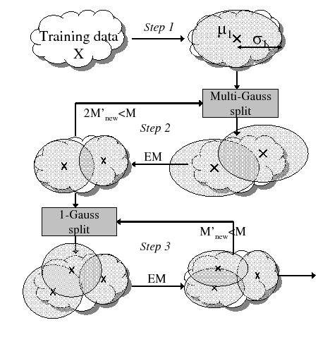
The introduced technique is inspired on the split and vanish
techniques used in the GMTK toolkit (Bilmes and Zweig, 2002) and the
mixture incrementing function in HTK. As seen in figure
3.7, the initial mean and variance of data ![]() are
computed in the same way as in the previous technique (step 1).
Then the algorithm iteratively splits each of the
are
computed in the same way as in the previous technique (step 1).
Then the algorithm iteratively splits each of the ![]() Gaussian mixtures into two mixtures, obtaining a total of
Gaussian mixtures into two mixtures, obtaining a total of
![]() mixtures, while
mixtures, while
![]() , the desired model
complexity. The
, the desired model
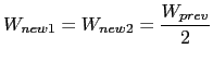
complexity. The ![]() Gaussian mixtures are computed from
their previous counterpart by
Gaussian mixtures are computed from
their previous counterpart by
After each split, a single step EM training of the current models
given data ![]() is performed to allow for the Gaussian mixtures to
adapt mean and variance to the data.
is performed to allow for the Gaussian mixtures to
adapt mean and variance to the data.
Once an extra splitting iteration would overpass the desired number of desired Gaussian mixtures, the algorithm moves into a single Gaussian split mode (step 3). In it the Gaussian selected to split is the one with the highest weight, and it is split in the same way as shown before. Some experiments were performed with different alternative splitting/vanishing procedures but to initialize GMM models with a small number of Gaussian mixtures it was seen that performance would diminish any time that vanishing was applied, therefore the technique applied here only uses a splitting procedure. Also, the defunct function implemented by HTK to discard Gaussians with low weigh was seen to be perjudicial for the GMM models grown here.
Once the number of initial cluster ![]() is defined, in the
broadcast news system it was explained how speaker clusters were
initialized by evenly assigning the available data into the
different clusters and doing several segmentation-training
iterations to allow for homogeneous data to cluster together.
While this mechanism is very simple and gives surprisingly good
results, it does not ensure that the final clusters contain only
data from one cluster (i.e. with a high purity).
is defined, in the
broadcast news system it was explained how speaker clusters were
initialized by evenly assigning the available data into the
different clusters and doing several segmentation-training
iterations to allow for homogeneous data to cluster together.
While this mechanism is very simple and gives surprisingly good
results, it does not ensure that the final clusters contain only
data from one cluster (i.e. with a high purity).
In order to improve on the linear initialization technique, several alternative methods were tested, including K-means at the segment level, E-HMM top-down clustering (Meignier et al., 2001) and others, finally designing a brand new algorithm that has been called the friends-and-enemies initialization and is further explained in section 4.2.1.